Analysis Jobs¶

NUPACK provides the capability to analyze equilibrium properties over one of two ensembles:

• Complex Analysis: analyze the equilibrium base-pairing properties of a complex of interacting nucleic acid strands [Dirks07,Fornace20].

• Test Tube Analysis: analyze the equilibrium concentrations and base-pairing properties for a test tube of interacting nucleic acid strands [Dirks07,Fornace20].

Note that a complex ensemble is subsidiary to a test tube ensemble, so complex analysis is inherent in test tube analysis (but not vice versa). As it is typically infeasible to experimentally study a single complex in isolation, we recommend analyzing nucleic acid strands in a test tube ensemble that contains the complex of interest as well as other competing complexes that might form in solution. For example, if one is experimentally studying strands A and B that are intended to predominantly form a secondary structure within the ensemble of complex A$\cdot$ B, one should not presuppose that the strands do indeed form A$\cdot$ B and simply analyze the base-pairing properties of that complex. Instead, it is more physically relevant to analyze a test tube ensemble containing strands A and B interacting to form multiple complex species (e.g., A, B, A$\cdot$A, A$\cdot$B, B$\cdot$B) so as to capture both concentration information (how much A$\cdot$B forms?) and structural information (what are the base-pairing properties of A$\cdot$B when it does form?).

NUPACK analysis algorithms enable simultaneous analysis of one or more test tube ensembles, providing significant cost savings if the same strands are present in more than one test tube. If for some reason, the test tube ensemble is not of interest for your application, NUPACK analysis algorithms also enable simultaneous analysis of one or more complex ensembles, providing significant cost savings if the same strands are present in more than one complex.

Specify a strand¶

A Strand is a single RNA or DNA molecule specified as a sequence and a strand name (keyword name):

A = Strand('AGUCUAGGAUUCGGCGUGGGUUAA', name='A') # name is required for strands
B = Strand('UUAACCCACGCCGAAUCCUAGACUCAAAGUAGUCUAGGAUUCGGCGUG', name='B')
C = Strand('AGUCUAGGAUUCGGCGUGGGUUAACACGCCGAAUCCUAGACUACUUUG', name='C')

A Strand sequence must contain only 'ACGTU'. Two strands are treated as indistinguishable only if they have the same name and the same sequence.

A Strand object supports a nt() method for calculating the number of nucleotides, for example:

A.nt() # --> 24

Specify a complex ensemble¶

A Complex of one or more interacting strands is specified as an ordered list of strands (i.e., an ordering of strands around a circle in a polymer graph) and an optional complex name (keyword name):

c1 = Complex([A]) # name is optional for complexes
c2 = Complex([A, B, B, C], name='ABBC')
c3 = Complex([A, A], name='AA')

In certain cases, it may be desirable to adjust the free energy of a complex (for example, if a protein is known to stabilize the complex). For such cases, the optional keyword bonus can be used to specify an additional free energy in kcal/mol (default: 0; negative value is stabilizing, postive value is destabilizing):

# destabilize c4 by 1 kcal/mol
c4 = Complex([A, B, C], name='ABC', bonus=+1.0)

# stabilize c5 by 10 kcal/mol
c5 = Complex([A, B], name='AB', bonus=-10.0)

Additional fields and methods are available for a Complex object:

• .strands: a tuple of strands
• .nstrands(): the number of strands in the complex
• .nt(): the number of nucleotides in the complex

For example:

c2.strands    # --> (<Strand A>, <Strand B>, <Strand B>, <Strand C>)
c2.nstrands() # --> 4
c2.nt()       # --> 168

Specify a test tube ensemble¶

A Tube is specified as a tube name (keyword name) and a set of strands (keyword strands), each introduced at a user-specified concentration (units of M), that interact to form a set of complexes (keyword complexes: defaults to the strand set). The set of complexes is optionally specified using SetSpec() in any of three ways:

• Combinatorially using keyword max_size to automatically generate the set of all complexes up to a specified number of strands (default: max_size=1).
• Using keyword include to include an explicitly specified set of complexes (default: None).
• Using keyword exclude to exclude an explicitly specified set of complexes (default: None).

For example:

t1 = Tube(strands={A: 1e-6, B: 1e-8}, name='t1') # complexes defaults to [A, B]

t2 = Tube(strands={A: 1e-6, B: 1e-8, C: 1e-12},
    complexes=SetSpec(max_size=3, include=[c2,[B, B, B, B]], exclude=[c1]),
    name='t2')

If desired, the complexes in a specified Tube can be queried as follows:

print(t1.complexes) # --> {<Complex A>, <Complex B>}
print(t2.complexes) # --> {<Complex (C+C+B)>, <Complex (B)>,
    # <Complex (A+C+B)>, <Complex (C+C+C)>, <Complex (C)>, <Complex (A+A+B)>,
    # <Complex (A+C)>, <Complex (B+B+B+B)>, <Complex (A+A)>, <Complex (A+B+B)>,
    # <Complex (B+B)>, <Complex (A+B)>, <Complex (B+B+B)>, <Complex (A+B+C)>,
    # <Complex (A+C+C)>, <Complex (A+A+A)>, <Complex (C+C)>, <Complex (A+A+C)>,
    # <Complex ABBC>, <Complex (C+B+B)>, <Complex (C+B)>}

Run a test tube analysis job¶

The tube_analysis command calculates the partition function, and equilibrium concentration, for each complex species $j$ in one or more test tube ensembles. The test tube ensembles to be analyzed are specified using the tubes keyword. If desired, a physical model is specified using the model keyword (otherwise the default physical model is used):

# specify strands
a = Strand('CUGAUCGAU', name='a')
b = Strand('GAUCGUAGUC', name='b')

# specify tubes
t1 = Tube(strands={a: 1e-8, b: 1e-9}, complexes=SetSpec(max_size=3), name='t1')
t2 = Tube(strands={a: 1e-10, b: 1e-9}, complexes=SetSpec(max_size=2), name='t2')

# analyze tubes
model1 = Model()
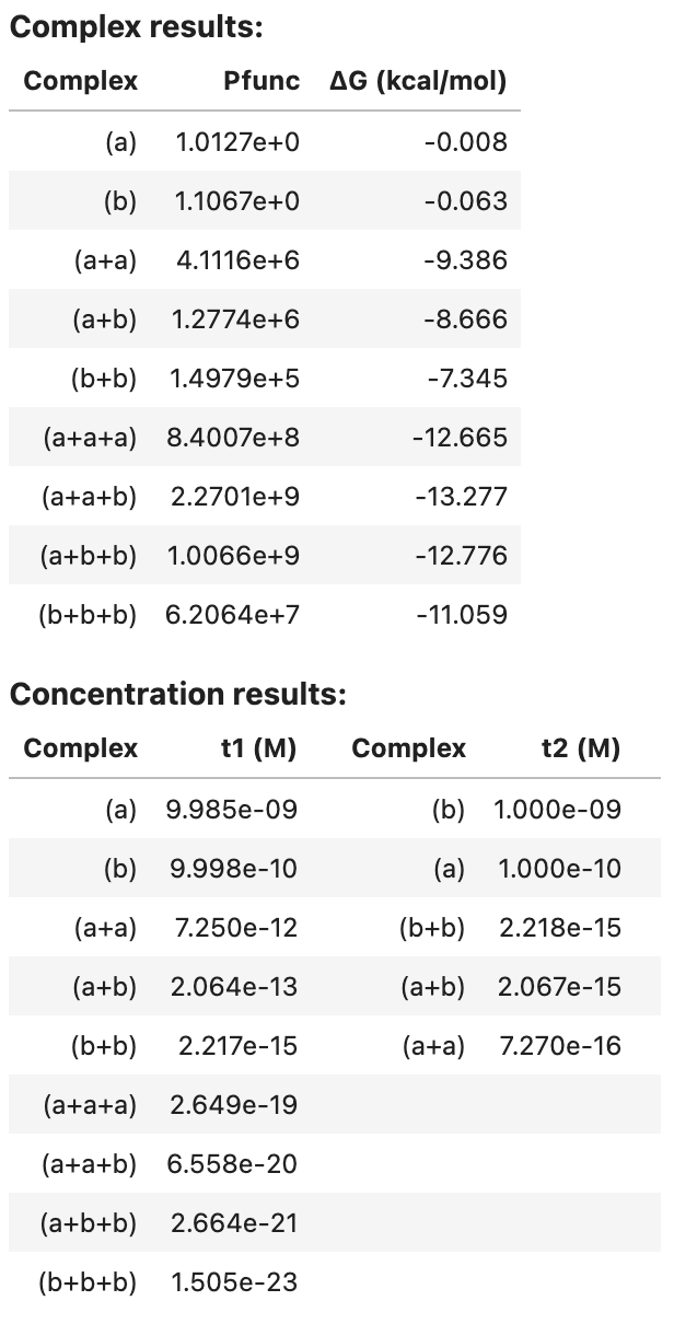
tube_results = tube_analysis(tubes=[t1, t2], model=model1)

tube_analysis returns an AnalysisResult object that can be viewed as a table in a Jupyter notebook, for example:

tube_results

For each complex in the ensemble, the partition function and complex free energy (units of kcal/mol) are displayed. For each tube, the equilibrium complex concentration of each complex in the tube is displayed (units of M).

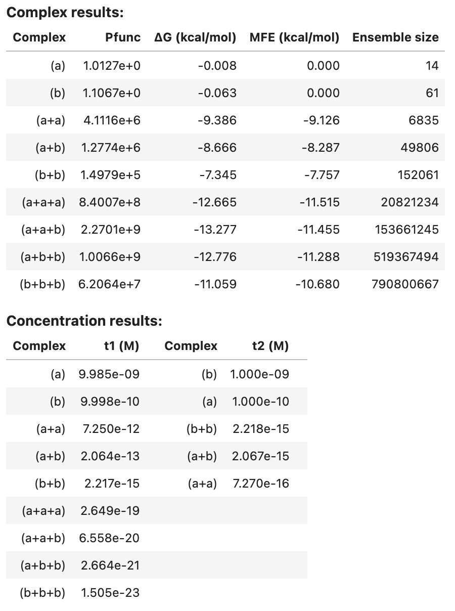
Optionally, additional quantities are calculated for each complex in the specified tubes (see Job Options). For example, additionally calculate equilibrium base-pairing probabilities, the MFE proxy structure(s), 100 Boltzmann-sampled structures, and the ensemble size for each complex in the tube:

model1 = Model()
tube_results2 = tube_analysis(tubes=[t1, t2], model=model1,
    compute=['pairs', 'mfe', 'sample', 'ensemble_size'],
    options={'num_sample': 100}) # max_size=1 default

tube_results2

Note that pairs and sample results are too large to be included in the summary table. See below for programmatic access to these results.

Specify a set of complexes¶

A ComplexSet is specified as a set of strands (keyword strands) that interact to form a set of complexes (keyword complexes: defaults to the strand set). The set of complexes is optionally specified using SetSpec() in any of three ways:

• Combinatorially using keyword max_size to automatically generate the set of all complexes up to a specified number of strands (default: max_size=1).
• Using keyword include to include an explicitly specified set of complexes (default: None).
• Using keyword exclude to exclude an explicitly specified set of complexes (default: None).

For example:

set1 = ComplexSet(strands=[A, B, C]) # complexes defaults to [[A], [B], [C]]

set2 = ComplexSet(strands=[A, B, C],
    complexes=SetSpec(max_size=3, include=[c2, [B, B, B, B]], exclude=[c1]))

Run a complex analysis job¶

The complex_analysis command calculates one or more physical quantities (see Job Options) for each complex in a ComplexSet:

# specify strands
a = Strand('CUGAUCGAU', name='a')
b = Strand('GAUCGUAGUC', name='b')

# specify complex set
set1 = ComplexSet(strands=[a, b], complexes=SetSpec(max_size=3))

# calculate the partition function for each complex in the complex set
model1 = Model()
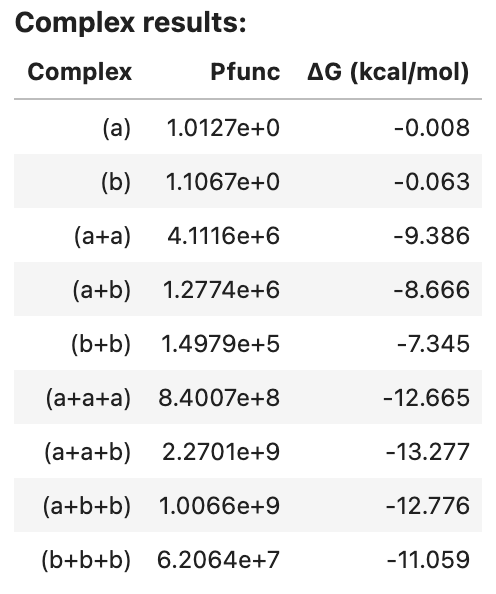
complex_results1 = complex_analysis(complexes=set1, model=model1, compute=['pfunc'])

complex_analysis returns an AnalysisResult object that can be viewed as a table in a Jupyter notebook, for example:

complex_results1

Output:

If desired, a Tube can be specified in place of a ComplexSet, in which case the strand concentrations are ignored since complex_analysis does not calculate equilibrium complex concentrations, and hence does not require concentration information for the strand species. For example:

# specify strands
a = Strand('CUGAUCGAU', name='a')
b = Strand('GAUCGUAGUC', name='b')

# specify tube
tube1 = Tube(strands={a:1e-8, b:1e-10}, complexes=SetSpec(max_size=3), name='tube1')

# calculate the partition function for each complex in the tube
model1 = Model()
complex_results2 = complex_analysis(complexes=tube1, model=model1, compute=['pfunc'])

Run a complex concentrations job¶

Use the complex_concentrations command to calculate the equilibrium concentration of each complex in a test tube ensemble (keyword tube) using the AnalysisResult data (keyword data) from a previous call to complex_analysis (which at minimum must contain the partition function for each complex). The tube ensemble can be specified either using Tube (which specifies strand concentrations) or as a ComplexSet, in which case the strand concentrations must additionally be specified (keyword concentrations):

 # specify strand concentrations for ComplexSet set1
concentration_results1 = complex_concentrations(tube=set1, data=complex_results1,
    concentrations={a: 1e-8, b: 1e-8})

# use strand concentrations previously specified for tube1
concentration_results2 = complex_concentrations(tube=tube1, data=complex_results2)

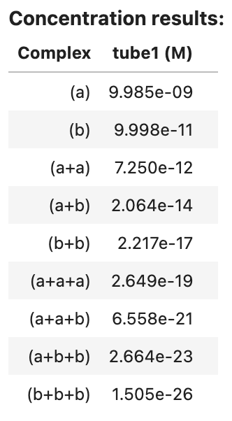
complex_concentrations returns an AnalysisResult object that can be viewed as a table in a Jupyter notebook, for example:

concentration_results2

Output:

Job options¶

The compute keyword is optional for tube_analysis (default: 'pfunc') and required for complex_analysis (no default), specifying a list of strings denoting calculations to be performed for each complex [Fornace20]:

• 'pfunc': calculate the partition function.

• 'pairs': calculate the matrix of equilibrium base-pairing probabilities. If 'pairs' is specified, tube_analysis or complex_concentrations will further calculate the matrix of test tube ensemble pair fractions. See the sparsity_fraction and sparsity_threshold options below.

• 'sample': calculate a set of Boltzmann-sampled structures from the complex ensemble. See option num_sample below.

• 'mfe': calculate the MFE proxy structure, the free energy of the MFE proxy secondary structure and the free energy of the MFE stacking state. If there is more than one MFE stacking state, the algorithm returns a list of the corresponding MFE proxy secondary structures, each with the free energy of the MFE proxy secondary structure and with the (same) free energy of the MFE stacking state.

• 'subopt': calculate the set of suboptimal proxy structures with a stacking state within a specified free energy gap of the MFE stacking state. The algorithm returns a list of suboptimal proxy secondary strutures, each with the free energy of the MFE proxy secondary structure, and with the free energy of its lowest-energy stacking state that falls within the energy gap. See option subopt_gap below.

• 'ensemble_size': calculate the complex ensemble size in terms of either the number of secondary structures (if using a physical model with nostacking) or the number of stacking states (if using a physical model with stacking).

The optional options keyword specifies options that modify the calculations performed for each complex:

• 'sparsity_fraction': f can be used in conjuction with 'pairs' to return a sparse matrix containing the fraction f of the largest pair probabilities for each base (default 'sparsity': 1 returns the full pair probability matrix).

• 'sparsity_threshold': t can be used in conjuction with 'pairs' to return a sparse matrix containing the only pair probabilities greater than or equal to t (default 'sparsity_threshold': 0 returns the full pair probability matrix).

• 'num_sample': n can be used in conjunction with 'sample' to specify the number of structures to be sampled (default 'num_sample': 1).

• 'subopt_gap': g can be used in conjunction with 'subopt' to specify the (non-negative) free energy gap in kcal/mol (default 'subopt_gap': 0).

By default, NUPACK analysis jobs run in parallel.

Job results¶

Scalar results of NUPACK analysis jobs can be conveniently displayed as a table, printed as text, or introspected programmatically. Consider the following test tube analysis job:

a = Strand('CCG', name='a')
b = Strand('CGG', name='b')
c = Complex([a, b], name='c')

t1 = Tube({a: 1e-6, b: 1e-9}, complexes=SetSpec(max_size=2, include=[c]), name='t1')
t2 = Tube({a: 1e-8, b: 1e-9}, complexes=SetSpec(include=[c]), name='t2')

my_model = Model()
my_result = tube_analysis([t1, t2], model=my_model,
    compute=['pfunc', 'pairs', 'mfe', 'sample', 'subopt'],
    options={'num_sample': 2, 'energy_gap': 0.5})

Tabular display¶

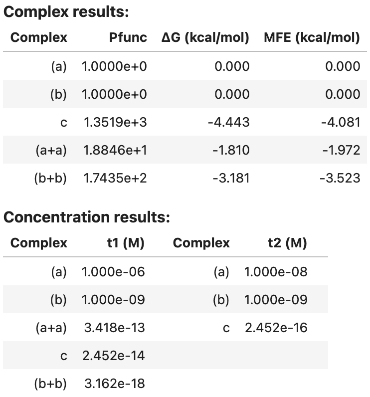
You can display a summary table of results in a Jupyter notebook, for example:

my_result

Output:

Textual display¶

You can view an ASCII representation of the same data by using the print function:

print(my_result)

Output:

Complex results:
  Complex      Pfunc dG (kcal/mol) MFE (kcal/mol)
0     (a)  1.0000e+0         0.000          0.000
1     (b)  1.0000e+0         0.000          0.000
2       c  1.3519e+3        -4.443         -4.081
3   (a+a)  1.8846e+1        -1.810         -1.972
4   (b+b)  1.7435e+2        -3.181         -3.523
Concentration results:
Complex    t1 (M)   Complex    t2 (M)
    (a) 1.000e-06       (a) 1.000e-08
    (b) 1.000e-09       (b) 1.000e-09
  (a+a) 3.418e-13         c 2.452e-16
      c 2.452e-14
  (b+b) 3.162e-18

For convenience, you can print the identical ASCII result to a text file using the save_text function:

my_result.save_text('my_result.txt')

Programmatic access¶

More detailed results can also be displayed by programmatic access into an AnalysisResult object. This class contains two fields:

• .complexes: a Python dict mapping each Complex to a ComplexResult
• .tubes: a Python dict mapping each Tube to a TubeResult

The information contained in these two fields depends on which type of analysis calculation was performed:

• For tube_analysis, the .tubes and .complexes fields are both non-empty.
• For complex_analysis, only the .complexes field is non-empty.
• For complex_concentrations, only the .tubes field is non-empty.

For convenience, you can index into an AnalysisResult via a Complex or Tube identifier (or via the assigned or auto-generated name of a Complex or Tube) as described in the following two sections.

Results for individual complexes¶

You can index into AnalysisResult object via a Complex identifier (or via the name of a Complex) to get a ComplexResult object containing all the complex ensemble quantities that were calculated in a tube_analysis or complex_analysis calculation. A ComplexResult contains the following fields (if a quantity was not computed, the field is set to None):

• pfunc: the complex partition function (held as a decimal.Decimal; convert to a float via float(pf) or calculate the logarithm via float(pf.log())).
• free_energy: the complex free energy in kcal/mol (held as a float).
• pairs: the matrix of equilibrium base-pairing probabilities (held as a PairsMatrix object containing a .to_array() method for conversion to numpy as illustrated below).
• sample: a list of Boltzmann-sampled structures, each an instance of a Structure object.
• mfe: a list of MFE proxy structures. Each entry contains fields .structure, .energy, and .stack_energy. .energy is the free energy of the MFE proxy secondary structure, while .stack_energy is the free energy of the MFE stacking state.
• subopt: a list of suboptimal proxy structures. Each entry contains fields .structure, .energy, and .stack_energy. .energy is the free energy of the MFE proxy secondary structure, while .stack_energy is the free energy of its lowest-energy stacking state that falls within the energy gap.
• ensemble_size: the complex ensemble size (held as int) representing either the number of secondary structures (if using a physical model with nostacking) or the number of stacking states (if using a physical model with stacking).
• model: the Model that was used for the analysis calculation.

For example, we can index the AnalysisResult object my_result with complex c (or by its name 'c') to obtain a ComplexResult object c_result that enables printing of specific physical quantities for that complex:

c_result = my_result[c] # equivalent to my_result['c']
print('Physical quantities for complex c')
print('Complex free energy: %.2f kcal/mol' % c_result.free_energy)
print('Partition function: %.2e' % c_result.pfunc)
print('MFE proxy structure: %s' % c_result.mfe[0].structure)
print('Free energy of MFE proxy structure: %.2f kcal/mol' % c_result.mfe[0].energy)
print('Equilibrium pair probabilities: \n%s' % c_result.pairs)

Output:

Physical quantities for complex c
Complex free energy: -4.44 kcal/mol
Partition function: 1.35e+03
MFE proxy structure: (((+)))
Free energy of MFE proxy structure: -4.08 kcal/mol
Equilibrium pair probabilities:
[[0.1000 0.0000 0.0000 0.0000 0.0061 0.8938]
 [0.0000 0.0083 0.0000 0.0000 0.9873 0.0044]
 [0.0000 0.0000 0.3839 0.6161 0.0000 0.0000]
 [0.0000 0.0000 0.6161 0.3839 0.0000 0.0000]
 [0.0061 0.9873 0.0000 0.0000 0.0066 0.0000]
 [0.8938 0.0044 0.0000 0.0000 0.0000 0.1018]]

aa_result = my_result['(a+a)']

If desired, the MFE proxy structure can be represented as a structure matrix of zeros and ones:

c_result = my_result[c]
print('MFE proxy structure:\n%s' % c_result.mfe[0].structure.matrix())

Output:

MFE proxy structure:
[[0 0 0 0 0 1]
 [0 0 0 0 1 0]
 [0 0 0 1 0 0]
 [0 0 1 0 0 0]
 [0 1 0 0 0 0]
 [1 0 0 0 0 0]]

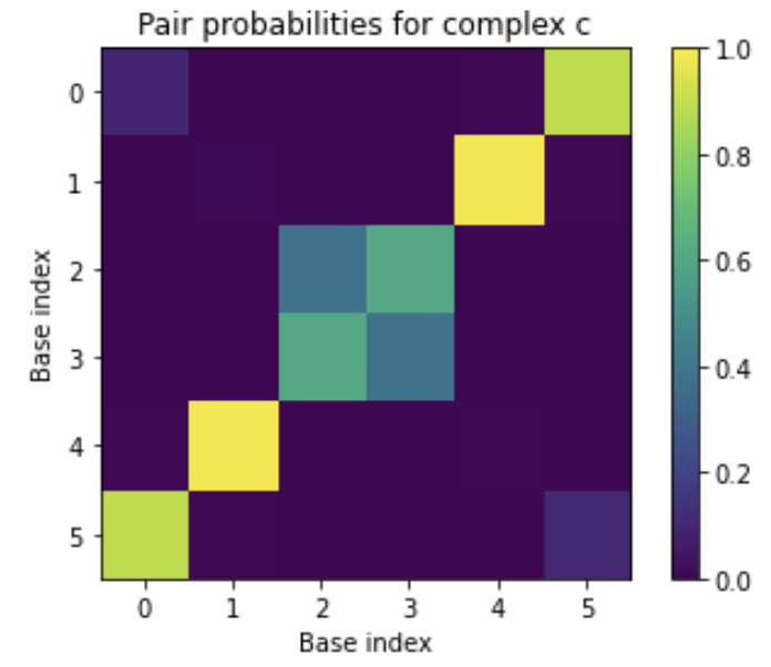
The equilibrium pair probability matrix is returned as a PairsMatrix object, which can be converted to a numpy array via the to_array() method for display in a Jupyter notebook:

import matplotlib.pyplot as plt

plt.imshow(my_result[c].pairs.to_array())
plt.xlabel('Base index')
plt.ylabel('Base index')
plt.title('Pair probabilities for complex c')
plt.colorbar()
plt.clim(0, 1)
plt.savefig('my-figure.pdf') # optionally, save a PDF of your figure

Output:

For some use cases, you may wish to convert a PairsMatrix to a scipy matrix via the to_sparse() method.

It is straightforward to collect information across complexes in an AnalysisResult object. Since my_result.complexes is an ordinary python dict, iterating through its .items() enables collection of each complex result. For example, to operate on the equilibrium pair probability matrix for each complex in my_result:

import numpy as np

for my_complex, complex_result in my_result.complexes.items():
    P = complex_result.pairs.to_array()
    s = 'Expected number of unpaired nucleotides at equilibrium in complex %s = %.2f'
    print(s % (my_complex.name, np.diagonal(P).sum()))

Output:

Expected number of unpaired nucleotides at equilibrium in complex c = 0.98
Expected number of unpaired nucleotides at equilibrium in complex (b) = 3.00
Expected number of unpaired nucleotides at equilibrium in complex (a+a) = 2.70
Expected number of unpaired nucleotides at equilibrium in complex (b+b) = 2.25
Expected number of unpaired nucleotides at equilibrium in complex (a) = 3.00

To collect a dict of MFEs for each complex:

my_mfes = {my_complex.name: complex_result.mfe[0].energy
    for my_complex, complex_result in my_result.complexes.items()}
print(my_mfes)

Output:

{'c': -4.081351280212402, '(b)': 0.0, '(a+a)': -1.9719057083129883, '(b+b)': -3.5225014686584473, '(a)': 0.0}

To print out the complex concentrations for a given tube:

for my_complex, conc in my_result.tubes[t1].complex_concentrations.items():
    print('The equilibrium concentration of %s is %.2e M' % (my_complex.name, conc))

Output:

The equilibrium concentration of c is 2.45e-14 M
The equilibrium concentration of (b) is 1.00e-09 M
The equilibrium concentration of (a+a) is 3.42e-13 M
The equilibrium concentration of (b+b) is 3.16e-18 M
The equilibrium concentration of (a) is 1.00e-06 M

Results for individual test tubes¶

You can index into an AnalysisResult object via a Tube identifier (or via the name of a Tube) to get a TubeResult object containing all the tube ensemble quantities that were calculated in a tube_analysis or complex_concentrations calculation. This class contains the following fields:

• complex_concentrations: a dict from Complex to its equilibrium concentration in molar (held as a float).
• fraction_bases_unpaired: a float in $[0,1]$ denoting the equilibrium fraction of nucleotides that are unpaired in the test tube ensemble.
• ensemble_pair_fractions: a square matrix of test tube ensemble pair fractions. Row and column indices refer to the concatenated base index formed by concatenating the strands of the input Tube (in order). This field is None if pair probabilities were not calculated (i.e., if option pairs was not specified for the tube_analysis or complex_analysis job).

Concentrations may be printed as follows:

t1_result = my_result[t1] # equivalent to my_result['t1']
for my_complex, conc in t1_result.complex_concentrations.items():
    print('The equilibrium concentration of %s is %.3e M' % (my_complex.name, conc))

Output:

The equilibrium concentration of c is 2.452e-14 M
The equilibrium concentration of (b) is 1.000e-09 M
The equilibrium concentration of (a+a) is 3.418e-13 M
The equilibrium concentration of (b+b) is 3.162e-18 M
The equilibrium concentration of (a) is 1.000e-06 M

Test tube ensemble pair fractions may be printed as follows:

print(t1_result.ensemble_pair_fractions)

Output:

[[1.0000 0.0000 0.0000 0.0000 0.0000 0.0000]
 [0.0000 1.0000 0.0000 0.0000 0.0000 0.0000]
 [0.0000 0.0000 1.0000 0.0000 0.0000 0.0000]
 [0.0000 0.0000 0.0000 1.0000 0.0000 0.0000]
 [0.0000 0.0000 0.0000 0.0000 1.0000 0.0000]
 [0.0000 0.0000 0.0000 0.0000 0.0000 1.0000]]

Saving a job summary¶

To save a textual job summary using the save_text method:

my_result.save_text('my-result.txt')

Saving and reloading job results¶

Save an AnalysisResult as a binary file using the save method:

my_result.save('my-result.o')

to enable reloading during a future session using the load method:

my_result = AnalysisResult.load('my-result.o')

This functionality uses Python’s built-in pickle module.